
Quick answer
Heteroscedasticity means that a regression’s error variance changes with the predictors, groups or time. A widening residual cloud is one example. If the conditional mean is correctly specified and the errors are exogenous, unequal variance alone does not bias OLS coefficients; it can make the usual standard errors and confidence intervals unreliable. Diagnose the pattern, then choose inference, weighting or a variance model to match your goal.
- Check the spread of residuals across fitted values, individual predictors, groups and time. A Q–Q plot answers a different question.
- OLS with HC3 keeps the coefficients and predictions unchanged. It changes their estimated uncertainty.
- Robust standard errors can be smaller as well as larger. Our checked example shows both.
- HC3, HAC, clustered covariance and volatility models address different data structures; they are not interchangeable.
- The complete synthetic experiment, CSV, plots and exact results are freely downloadable below.
What heteroscedasticity means
Suppose you predict spending from income. Two people with the same income can spend different amounts, so your regression has an error term. If that unexplained spending varies much more among high-income households than among low-income households, the error variance depends on income. That is heteroscedasticity. The example is an illustration, not a claim about a particular household dataset.
For a linear model, write yᵢ = xᵢ′β + εᵢ. Homoscedasticity means Var(εᵢ | X) = σ² for every observation. Heteroscedasticity means that some of those conditional variances differ. Conditioning matters: a response can have a wide overall range simply because its mean changes with a predictor. That alone does not establish unequal error variance.
Errors are unobserved deviations from the population model. Residuals are the fitted sample’s observed deviations, eᵢ = yᵢ − ŷᵢ. We use residual plots and tests to investigate the errors, but residuals are not literally independent draws from that population distribution. Fitting coefficients imposes constraints on them, and high-leverage observations change their variability.
Both heteroscedasticity and heteroskedasticity are accepted spellings. In regression, “unequal conditional error variance” is the useful meaning. A visible trend in the average residual is a separate warning about the conditional mean; an expanding spread around zero is a warning about conditional variance.
Homoscedasticity vs heteroscedasticity
Scroll horizontally to read every column.
| Question | Homoscedastic errors | Heteroscedastic errors |
|---|---|---|
| Conditional variance | One common variance | Variance changes across observations |
| Typical residual cloud | Similar width across predictors | Width may widen, narrow, cycle or differ by group |
| OLS coefficients with a correct mean and exogeneity | Unbiased under the usual finite-sample conditions | Still unbiased under those same conditions |
| Efficiency | OLS is BLUE if the other Gauss–Markov conditions hold | OLS need not be the most efficient linear unbiased estimator |
| Conventional covariance formula | Appropriate under its other assumptions | Generally inappropriate |
| Main next step | Check the remaining assumptions | Match the remedy to the variance and dependence structure |
Do not read “unbiased” as “this fitted coefficient equals the truth.” Unbiasedness describes repeated samples under assumptions. Any one fitted coefficient can be far from the population parameter.
Homoscedasticity also does not imply normality or independence. Independent errors can have different variances; errors with equal variances can be serially correlated. A bell-shaped pooled residual histogram can hide unequal spread within groups. Those are different questions and require different checks.
Read four residual patterns, not just a funnel
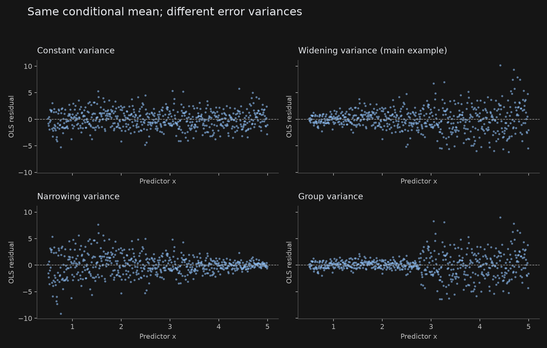
These plots use 600 synthetic observations, the same conditional mean and the same seeded innovations. Only the error standard deviation changes. They are generated by the downloadable script, rather than drawn to suggest a particular market result.
- Constant variance: the cloud has roughly similar thickness. Individual extreme residuals are possible even under constant variance.
- Widening variance: residual magnitude tends to increase as x increases. This is the textbook funnel, but it is only one possible pattern.
- Narrowing variance: large errors concentrate at low x. Heteroscedasticity can run in either direction.
- Group variance: the spread changes at the boundary between two groups. A smooth funnel is unnecessary.
Compare residuals with fitted values, then with each important predictor. In multiple regression, the fitted value compresses several dimensions, so a predictor-specific variance pattern can disappear in the first plot. Use meaningful groups or calendar segments when those are plausible variance drivers.
A curved band whose centre rises and falls suggests that the mean function is misspecified. An expanding band whose centre stays near zero suggests a variance issue. Both can occur at once. Inspect leverage and influence before deciding whether one unusual point or a broader process drives the appearance.
A scale-location plot, typically the square root of absolute standardized residuals against fitted values, makes changing spread easier to see. A Q–Q plot instead examines distributional shape. Neither a straight Q–Q plot nor a high R² certifies constant variance. NIST’s graphical example and Wisconsin’s diagnostics walkthrough give further visual context.
What changes in OLS, and what does not
OLS chooses coefficients to minimize the sum of squared residuals. Computing those coefficients does not require constant variance. In a full-rank linear model with E(ε | X) = 0, unequal variance alone does not introduce coefficient bias.
Conventional OLS uncertainty estimates use σ²(X′X)⁻¹. With unequal error variance, the conditional covariance instead involves (X′X)⁻¹ X′ΩX (X′X)⁻¹, where Ω contains the errors’ variances and, if present, their covariances. Using the constant-variance formula in that setting can misstate a coefficient’s precision.
The direction is not always downward. Depending on the design and which coefficient you inspect, a conventional standard error can be too small or too large. That can lead to confidence intervals with the wrong coverage and hypothesis tests that reject too often or too rarely.
An HC covariance estimator estimates a sandwich covariance while retaining the OLS coefficients. It cannot repair an omitted-variable bias, reverse causality, a wrong target variable or an incorrectly specified mean. Those problems can violate exogeneity or change what the coefficient means.
Nor does an HC coefficient confidence interval provide a complete prediction interval for a new observation. Prediction uncertainty includes the new observation’s conditional noise variance. If that varies by x, an interval based on one pooled residual variance may be too narrow in noisy regions and too wide in quiet regions.
Finally, homoscedasticity is not required to build a useful predictor. For a prediction task, evaluate held-out error, subgroup performance and interval calibration. For an explanatory task, justify the identifying assumptions and the chosen uncertainty estimate. The statistical goal determines which consequence is most important.
Why unequal variance appears
Some variance patterns belong to the phenomenon being studied. Others point to measurement or modeling choices. Start with an explanation you can investigate.
Scroll horizontally to read every column.
| Possible driver | What to inspect | What the observation does not establish |
|---|---|---|
| Scale-dependent noise | Residual magnitude versus size, income or exposure | A large response range alone proves nothing about conditional variance |
| Different measurement quality | Instrument, source, subgroup or reporting precision | More rows in one group do not by themselves create different population variances |
| Omitted curvature or interaction | Residual mean versus fitted values and predictors | Robust covariance does not correct the wrong mean |
| A few high-leverage observations | Influence measures and sensitivity analysis | Removing inconvenient points is not an automatic remedy |
| Time-varying volatility | Residuals and squared residuals in date order | Heteroscedasticity alone does not prove serial correlation in the signed errors |
| Structural change | Business conditions, definitions and subperiod stability | One variance estimator cannot make a changing relationship stable |
A model for absolute transaction volumes may need a different variance structure from a model for percentage growth. Changing to a rate or a logarithm changes the question being answered. Treat it as a substantive modeling decision, then check the new model.
For financial time series, distinguish changing volatility from a predictable conditional mean. Returns can have little signed autocorrelation while their squares show persistent dependence. A variance model addresses that volatility pattern; it does not establish a profitable directional forecast.
A practical diagnostic workflow
- Check the input and sampling structure. Record the target’s units, missing-data treatment, time ordering and whether observations share a person, firm, date or site. Duplicate rows and inconsistent units can manufacture apparent patterns.
- Fit a defensible mean model. Inspect residual centres, transformations and relevant interactions. A heteroscedasticity test is difficult to interpret if obvious curvature remains.
- Plot spread in several views. Use residuals versus fitted values, key predictors, meaningful groups and time. Inspect standardized residuals and leverage too.
- Choose a test and state its alternative. Decide which variables plausibly explain variance before repeatedly testing arbitrary combinations.
- Choose covariance or estimation for the goal. Independent observations may call for HC3; serial dependence may call for HAC; within-group dependence may call for clustering. A well-supported variance model may justify weighting.
- Report assumptions and sensitivity. Record the design, sample size, test variant, covariance method, uncertainty convention and meaningful alternative specifications.
The test does not choose your final model for you. A p-value greater than 0.05 means that this test did not detect its alternative at that threshold. It does not certify homoscedasticity. Small samples, limited variation in the variance predictors and unsuitable alternatives can all limit power.
Conversely, a very large sample can detect small departures from constant variance. Assess their practical effect on the inference you care about. Choose a covariance method based on the design instead of toggling between “ordinary” and “robust” solely to obtain a desired p-value.
Breusch–Pagan, White and Goldfeld–Quandt tests
Scroll horizontally to read every column.
| Test | Main idea | Useful when | Important limitation |
|---|---|---|---|
| Breusch–Pagan / Koenker version | Relate squared residuals to selected variance predictors | You have a small, motivated variance specification | Can miss alternatives outside that specification |
| White | Include squares and interactions in an auxiliary variance regression | You want broader polynomial alternatives | Many regressors consume degrees of freedom; it is not sensitive to every possible pattern |
| Goldfeld–Quandt | Compare residual variances in two ordered subsamples | There is a prespecified variable along which variance may change | Ordering, split, dropped observations and alternative affect the result |
For the Koenker Breusch–Pagan variant (robust=True) and the White test used below, the LM statistic is n × R² from an auxiliary regression. Its large-sample reference distribution is chi-squared with degrees of freedom determined by the independent auxiliary regressors excluding the intercept. Include an intercept and inspect rank when building the design. The original Breusch–Pagan variant (robust=False) instead uses half the explained sum of squares after normalizing squared residuals by their mean; do not apply the n × R² formula unchanged when switching variants. Official implementation.
In statsmodels, het_breuschpagan(..., robust=True) uses the Koenker variant. Here “robust” describes the test variant’s treatment of normality; it does not mean the regression has HC3 standard errors. The original Breusch–Pagan variant is available with robust=False and has a stronger normality assumption. Both still depend on suitable sampling conditions. Official test reference.
het_white constructs squared and interaction terms from the supplied explanatory variables, including a constant. Its LM and F outputs are alternative summaries of the auxiliary regression. A reported F p-value can be informative in finite samples; it is not a guarantee of exact small-sample validity under arbitrary heteroscedasticity. White test reference.
For Goldfeld–Quandt, compare residual mean squares with their degrees of freedom, not an arbitrary ratio of raw residual sums of squares. Sorting by a predictor, dropping a middle segment and selecting an increasing, decreasing or two-sided alternative are choices to report. If the scientific concern is group dependence or ARCH effects, use methods designed for those questions instead of treating every rejection as the same problem.
Run a complete, reproducible Python example
This synthetic experiment makes the ground truth explicit. The conditional mean is 2 + 0.8x; the error standard deviation is 0.3 + 0.65x; therefore its variance is (0.3 + 0.65x)². Distinguishing standard deviation from variance avoids a common simulation error.
Download the complete Python script, the exact 600-row CSV, and the machine-readable results. The script also regenerates the four-panel figure. It reads no external dataset.
The core calculation is below. Run it in a local Python environment with NumPy and statsmodels installed. The complete script also uses SciPy and Matplotlib. Our checked run used Python 3.14.0, NumPy 2.5.3, SciPy 1.18.1, statsmodels 0.15.0 and Matplotlib 3.11.2. Small floating-point differences across environments are possible.
import numpy as np
import statsmodels.api as sm
from statsmodels.stats.diagnostic import het_breuschpagan, het_white

rng = np.random.default_rng(20261003)
x = np.linspace(0.5, 5.0, 600)
X = sm.add_constant(x)
sigma = 0.3 + 0.65 * x
y = 2.0 + 0.8 * x + sigma * rng.standard_normal(len(x))

ols = sm.OLS(y, X).fit()
hc3 = ols.get_robustcov_results(cov_type="HC3", use_t=True)
wls = sm.WLS(y, X, weights=1.0 / sigma**2).fit()

assert np.allclose(ols.params, hc3.params)
assert np.allclose(ols.fittedvalues, hc3.fittedvalues)

for name, model in [("OLS", ols), ("HC3", hc3), ("WLS", wls)]:
    print(name, "coef", np.round(model.params, 6),
          "SE", np.round(model.bse, 6),
          "CI", np.round(model.conf_int(), 6))
print("Koenker BP:", het_breuschpagan(ols.resid, X, robust=True))
print("White:", het_white(ols.resid, X))
The WLS weights are an oracle illustration: we know sigma because we generated the data. A real dataset does not hand you its true conditional standard deviations. Do not copy these weights into unrelated data, use 1/y² as a shortcut, or choose weights by looking at the preferred coefficient significance.
The use_t=True setting explicitly uses a t reference for the confidence intervals. HC3 changes covariance, while this option changes the inferential reference distribution. Robust-covariance defaults may otherwise use a normal reference. This is a reporting choice, not a claim of exact t-distributed statistics under arbitrary unequal variance.
Checked results: ordinary vs robust standard errors
Scroll horizontally to read every column.
| Estimator | Intercept | Intercept SE | Slope | Slope SE | Slope 95% interval |
|---|---|---|---|---|---|
| Ordinary OLS | 1.833530 | 0.207555 | 0.856886 | 0.068223 | [0.722900, 0.990871] |
| Same OLS, HC3 covariance, t reference | 1.833530 | 0.155403 | 0.856886 | 0.072461 | [0.714577, 0.999194] |
| Oracle WLS | 1.824910 | 0.103673 | 0.864323 | 0.054787 | [0.756724, 0.971922] |
The OLS coefficients do not move when you request HC3. In this sample, the intercept’s robust standard error decreases and the slope’s increases. “Robust errors are always larger” is false even in a simple widening-variance experiment.
Scroll horizontally to read every column.
| Diagnostic on the ordinary OLS residuals | LM statistic | LM p-value | Auxiliary F statistic | F p-value |
|---|---|---|---|---|
| Koenker Breusch–Pagan, predictor x and intercept | 73.617667 | 9.481226e−18 | 83.633819 | 9.243331e−19 |
| White, original design with automatic expansion | 76.363489 | 2.617454e−17 | 43.531154 | 2.250521e−18 |
Both tests reject constant variance in this deliberately heteroscedastic dataset. Their p-values are tiny, not literally zero. Scientific notation prevents rounding from suggesting an impossible exact value.
The true slope is 0.8, while this draw’s fitted slope is about 0.857. All three intervals happen to include 0.8. One sample cannot establish a method’s repeated-sampling coverage or efficiency. WLS is a different estimator and happens to have smaller standard errors here with known variance weights; that outcome does not establish that estimated weights will help in a real application.
For a coverage experiment, repeat the whole data generation and estimation many times, then count intervals containing the known slope. Do not redraw only the confidence interval or select the seed that produces the preferred conclusion. Save the seed, package versions and full procedure so the next person can check what was tested.
Choose the fix that matches your objective
Scroll horizontally to read every column.
| Objective and data structure | Candidate method | What it changes | What it leaves unresolved |
|---|---|---|---|
| Coefficient inference with independent observations and a defensible mean | HC covariance, often HC3 | Standard errors, tests and intervals | Coefficients, omitted-variable bias and new-observation variance |
| More efficient estimation with a defensible variance model | WLS / feasible GLS | Observation weights and usually coefficients | Wrong weights, dependence and wrong mean |
| A multiplicative relationship with a positive target | Log or another justified transformation | Target scale and coefficient interpretation | Zero/negative values and retransformation bias |
| Serially dependent regression errors | HAC covariance | Inference allowing selected lag dependence | Prediction noise, model instability and choice of bandwidth |
| Observations correlated within groups | Clustered covariance | Inference reflecting within-group dependence | Too few independent clusters and incorrect clustering level |
| Conditional volatility forecasting | ARCH/GARCH or another variance model | A model for evolving conditional variance | Directional return forecasting and automatic trading profitability |
HC3: Its leverage adjustment uses squared residuals divided by (1 − hᵢᵢ)² inside the sandwich covariance. It can be a sensible finite-sample choice when observations are independent. Extreme leverage, very small samples or a badly specified mean still require investigation. “HC3” does not mean robust regression against outliers; the OLS fit itself has not changed. HC3 implementation.
WLS: Use weights proportional to inverse variance, 1/σᵢ², not inverse standard deviation. Estimated weights create another modeling step; assess their stability and inspect weighted residuals. A fitted variance model can improve efficiency if its assumptions are reasonable, but weights can also worsen the result. NIST on weighting and transformations provides a practical worked context.
Transformations: Log-transform only when the target and question justify it. If y contains zero or negative observations, replacing them with a tiny positive constant changes the data and can distort the model. A justified alternative model, two-part model or carefully explained transformation may be needed. If the target is log y, exponentiating a fitted mean does not in general recover the conditional mean of y; account for the error distribution when converting back.
Dependence: HC3 addresses heterogeneous variances without automatically handling off-diagonal error covariances. Use HAC for motivated time dependence or clustering for shared shocks within a meaningful group. State the HAC lag length, time spacing or cluster definition. Few clusters make asymptotic approximations fragile. The statsmodels covariance reference documents the distinct options.
Financial time series: volatility, dependence and prediction
Imagine a regression of one asset’s returns on market returns. You want to distinguish three questions: is the mean relationship defensible, is the coefficient uncertainty estimated appropriately, and does the model forecast the next period’s volatility? They need different evidence.
Volatility clustering means that large absolute movements tend to occur near other large absolute movements. An ARCH/GARCH specification models conditional variance from previous shocks and variances. It is useful when the research task is variance forecasting or risk scaling, with a specified mean model and properly ordered data.
A GARCH variance equation is not the same operation as giving a cross-sectional regression robust standard errors. Nor does fitting a volatility model establish that a financial series is nonstationary. A process can have a stationary unconditional distribution and still have changing variance conditional on past observations.
If you estimate a factor coefficient using serially dependent errors, HC3 alone may understate or overstate uncertainty because it ignores their dependence. A motivated HAC estimator can address the regression-inference task without requiring a complete parametric volatility model. If many assets share daily market shocks, clustering may need to reflect the panel structure.
For forecasting, fit models only with information available before the forecast. Select the specification on a training/validation period, then assess held-out variance forecasts and prediction intervals. Record what residuals, returns or standardized innovations actually feed the variance equation. A smooth fitted volatility curve is not sufficient evidence of good future forecasts.
The same discipline applies to a trading interpretation. A statistically significant coefficient is not a cost-adjusted strategy return. Link signal timing, exposure, turnover and execution assumptions explicitly; the separate mean reversion guide works through that distinction.
Three solved checks before you report the regression
Check 1 — is the mean wrong or is variance unequal? Your residual plot has constant thickness, but the average residual forms a U-shaped curve. The first concern is a missing nonlinear term in the mean. Adding HC3 changes estimated uncertainty around the same misspecified coefficients; it does not flatten the curve. Fit a justified mean specification and inspect the residuals again.
Check 2 — which weights? Group A’s error standard deviation is 2 and group B’s is 6. Their variances are 4 and 36, so inverse-variance weights are 1/4 and 1/36. Group A receives nine times Group B’s weight, not three times. Multiplying all weights by the same positive constant leaves WLS coefficients unchanged. You still need a reason to trust those variance estimates.
Check 3 — what did “robust” change? OLS and HC3 report identical coefficients and R² but different p-values. That is expected: the fitted conditional mean stayed the same; the covariance estimate changed. If a different regression reports different coefficients, check whether the sample, formula, weights, outlier treatment or estimator also changed.
For your own research note, write a sentence with the unit of observation, model formula, sample size, covariance choice and reason. Then add the diagnostic that motivated it and the main unresolved assumption. A short account that another person can audit is more useful than writing “all regression assumptions passed.”
Frequently asked questions
What is heteroscedasticity in simple terms?
The unexplained errors around a regression’s fitted relationship have different amounts of spread for different predictor values, groups or times. It concerns conditional error variance, not simply whether the response has a large overall range.
Does heteroscedasticity bias OLS coefficients?
Unequal variance alone does not cause bias when the linear conditional mean is correctly specified, the design is full rank and the errors have conditional mean zero. Omitted variables or endogeneity can still bias coefficients; robust covariance cannot repair that.
What is the null hypothesis of a heteroscedasticity test?
For the Breusch–Pagan and White variance tests, the null is constant conditional error variance under the test’s other assumptions. A failure to reject is not proof of constant variance, and a rejection does not identify a unique cause.
Is a residual funnel the only sign?
No. Variance can decrease, change between groups or follow a more complicated pattern. Inspect residuals against fitted values, individual predictors, groups and time, while separating a changing residual mean from changing spread.
Do robust standard errors always increase?
No. They can be smaller or larger for a particular coefficient. In our checked dataset, HC3 reduces the intercept SE from 0.207555 to 0.155403 but increases the slope SE from 0.068223 to 0.072461.
Does HC3 fix autocorrelation?
HC3 is designed for heteroscedasticity without automatically allowing serial correlation. If the errors are dependent over time or within groups, consider a justified HAC or clustered covariance estimator and report its lag or grouping choices.
Can I always take the logarithm to fix it?
No. Logs require a positive target and change the model’s scale and interpretation. Replacing nonpositive observations with a tiny number changes the data. Recheck the model after a justified transformation and handle retransformation appropriately.
Can the Python example run in the browser playground?
The complete experiment uses NumPy, statsmodels, SciPy and Matplotlib in a local Python environment. The linked playground is useful for small calculations; this guide does not assume it has all those packages available.
Sources and methodology
Sources checked Oct 3, 2026. Original exercises and synthetic examples are identified in the text. Employer disclosures, catalog records and technical documentation retain their own dates and limitations.
- NIST: Scatter plot with heterogeneous variability
Primary technical handbook; residual interpretation and inverse-variance weighting.
- NIST: Accounting for nonconstant variation
Worked weighting and transformation context; choosing a variance model.
- University of Wisconsin SSCC: Homoscedasticity diagnostics
University walkthrough with residual plots, groups, scale-location plots and tests.
- statsmodels: Breusch–Pagan and Koenker test
Function inputs, robust=True variant, intercept and finite-sample caveats.
- statsmodels: White test
Automatic squares and interactions, LM/F outputs.
- statsmodels: HC3 standard errors
Leverage-adjusted sandwich covariance formula.
- statsmodels: Robust covariance options
HC, HAC and cluster methods; t versus normal reference.
- statsmodels: Weighted least squares notebook
Primary executable documentation for WLS and known versus estimated weights.