
Quick answer
Mean reversion describes a tendency for a variable to move toward a reference level after a deviation. “The spread mean reverted” describes an observed return toward that level; it does not establish a reliable or profitable trading rule. This guide starts with the language, derives the models, separates statistical tests from tradeable evidence, and gives a reproducible synthetic experiment that can succeed, fail after costs, or fail after a regime change.
- Identify what reverts: a price, return, spread, residual, volatility measure or valuation ratio. Their meanings and trading instruments differ.
- A moving average describes past observations. It does not prove that the next price will move toward it.
- For an AR(1) with 0 < phi < 1, the conditional gap decays as phi^h; half-life is log(0.5) / log(phi).
- ADF, cointegration tests and Hurst estimates answer different questions. A small p-value or a low Hurst estimate does not establish net profitability.
- Fit parameters on earlier observations, specify execution timing, account for every traded leg and hold out later data before making a performance claim.
- The downloadable example contains synthetic data, checked accounting and a failing regime. Its outputs are an explanation of research mechanics.
What does “mean reverted” mean?
Mean reversion is the tendency of a variable to move back toward a reference level after moving away from it. In a specified model, this usually means that its expected future deviation shrinks. An individual path can still move farther away, and the reference level can cease to be useful.
“The spread mean reverted” is a past-tense description: the spread moved back toward its estimated average. “A mean-reverting spread” describes a hypothesised property of the process. “A mean reversion strategy” names a trading rule designed around that hypothesis. These expressions should not be treated as interchangeable evidence.
Suppose a machine normally produces 100 units each hour. A temporary blockage reduces output to 80, repairs restore it to 96, and output settles near 100. The output has moved toward its established level. If the machine permanently loses a production line and its new normal becomes 80, waiting for 100 assumes a mechanism that no longer exists. A market can make the same distinction harder to observe.
For a financial example, an illustrative spread usually sits near $4. It widens to $7 and later falls to $4.50. The $3 initial deviation has fallen to $0.50, so saying that it “mean reverted” is reasonable. That observation does not tell you whether you could identify the move beforehand, obtain both fills, or profit after costs.
Choose the variable before choosing the average
The first research decision is the object being measured. A claim about volatility returning toward its usual range is different from a claim that a stock will revisit an old price. A return reverting toward zero does not imply that the accumulated price will fall back to its starting point.
Scroll horizontally to read every column.
| Variable | Possible reference | What would a reversal mean? | Essential distinction |
|---|---|---|---|
| Price level | Estimated equilibrium or trailing average | Price moves toward that level | Long-run growth can make an old level irrelevant |
| Return | A baseline expected return | An unusually large return is followed by a smaller or opposite return | Stationary returns can coexist with a nonstationary price |
| Pair spread | Fitted combination of two prices | The residual gap narrows | High price correlation alone does not establish stability |
| Volatility | Model-implied long-run level | Volatility falls after a spike or rises after a quiet period | An option or futures contract is a different tradeable object |
| Valuation ratio | A conditional historical range | Price, earnings, or both change the ratio | A ratio can normalize without a profitable price trade |
A reference must also have an information timestamp. A 20-observation moving average at close t includes that close; a signal calculated from it becomes available only after the needed data arrives. An average computed from the entire history includes future prices when used to explain earlier trades.
Moving averages create a further trap: they can catch up to the price. If the price rises to 120 and stays there, its trailing average eventually approaches 120. The gap closes even though a short position earns no reversal profit. Measure the actual tradeable price change as well as the change in the plotted gap.
An AR(1) example you can calculate by hand
An autoregressive model of order one, or AR(1), provides a precise version of the idea:
The model is X(t+1) = c + phi × X(t) + epsilon(t+1). Assume the future innovation has conditional mean zero and a constant finite variance. With |phi| < 1, the stable long-run mean is mu = c / (1 − phi). Subtracting mu gives X(t+1) − mu = phi × [X(t) − mu] + epsilon(t+1).
Take c = 10 and phi = 0.90. The mean is 100, not 10. If X(t) = 120, its next conditional expectation is 10 + 0.90 × 120 = 118. The expected gap shrinks from 20 to 18. Repeating the calculation gives an h-step conditional forecast of 100 + 20 × 0.90^h. After seven observations this is about 109.57; after ten, about 106.97.
The realized next value is 118 plus the innovation. An innovation of +5 gives 123, farther from the mean. Mean reversion concerns the conditional tendency, so one adverse observation does not refute the model. A long sequence of persistent deviations may instead suggest that its parameters or assumptions have failed.
For phi = 1, the model becomes a random walk, possibly with drift. There is no finite equilibrium from c / (1 − phi). For −1 < phi < 0, deviations alternate in sign while their expected magnitude decays; this is an oscillating process. For phi = 0, the next conditional mean is immediately c. The usual smooth, positive-persistence half-life interpretation needs 0 < phi < 1.
These calculations concern the specified model. Estimating phi = 0.90 from a small sample does not establish that the real process will keep that coefficient. See the authors’ autoregressive-model explanation for the underlying model and stationarity conditions.
Half-life, OU models and the time available to trade
For an AR(1) with 0 < phi < 1, solve phi^h = 0.5 to get half-life = log(0.5) / log(phi). With phi = 0.90 this is approximately 6.58 observations. If observations are daily, the unit is trading days; if they are hourly, it is hours. Replacing daily observations with five-minute bars changes the model and its units, rather than simply multiplying the same estimate.
The continuous-time Ornstein–Uhlenbeck, or OU, model writes dX = theta × (mu − X) × dt + sigma × dW, with theta > 0. Its conditional expected value after duration h is mu + [X(t) − mu] × exp(−theta × h). Half-life is log(2) / theta. For theta = 0.20 per day, mu = 100 and X(t) = 120, half-life is 3.47 days and the three-day conditional expectation is approximately 110.98. The OU setting is covered in MIT’s lecture on the Ornstein–Uhlenbeck semigroup.
The exact sampled OU coefficient is phi = exp(−theta × delta), where delta is the observation interval. A small-step approximation uses phi approximately equal to 1 − theta × delta. These are close only when the step is sufficiently small. In a regression of change on lagged level, lambda = phi − 1. Use log(0.5) / log(1 + lambda) for the discrete estimate; −log(2) / lambda is an approximation.
Half-life measures the decay of the conditional expected deviation. It is not the average time until the path first touches the mean, a promised holding period, or a stop-loss. A fast statistical decay can be exhausted before your fill; a slow decay can incur financing costs and large intervening losses. Check its stability across earlier windows and compare it with signal-to-fill delay and realistic holding constraints.
Under an ideal Gaussian OU model, roughly 95% of stationary observations fall within two stationary standard deviations of the mean. That distributional coverage is not a 95% probability of returning to the mean before your exit deadline. A crossing probability requires a first-passage calculation, including the initial state, horizon and model parameters. Estimation uncertainty and changing regimes add further uncertainty.
Mean reversion, trend and momentum are different claims
Mean reversion trades toward a reference. Momentum trades in the direction of a measured prior move. A trend describes an evolving level or direction; a price can fluctuate around a rising trend while its deviations from that trend revert. The same instrument can exhibit different behaviour at different horizons.
Scroll horizontally to read every column.
| Research question | Mean reversion rule | Momentum rule |
|---|---|---|
| What predicts the next move? | A displacement from a specified reference | A specified past return or trend signal |
| Illustrative long entry | Negative residual below a threshold | Positive trailing return above a threshold |
| Main evidence needed | Conditional correction of the displacement | Conditional continuation of the measured move |
| Typical invalidation | Reference breaks or correction disappears | Continuation disappears or repeatedly reverses |
| Timing test | Does correction survive execution delay? | Does continuation survive execution delay? |
An oversold oscillator is not evidence that continuation has stopped. Likewise, an upward-sloping average does not show that every pullback should be bought. Specify the horizon and the variable, then compare both hypotheses on the same time-ordered data and cost assumptions.
Combining the two families also needs evidence. Similar exposures, common crisis losses and different trading costs can make a seemingly complementary combination less useful than expected. Our momentum research project uses synthetic teaching data and requires Pro access; its workflow provides a separate place to practise the timing and holdout comparison. The experiment below is fully available here.
How to test mean reversion without overstating the result
Start with an economic or mechanical reason for correction and a plot of the chosen variable. Check missing data, splits, stale quotes, seasonality and abrupt level changes. A numerical test on a mishandled price series can produce a precise answer to the wrong question.
Stationarity means that specified distributional properties remain stable through time; covariance stationarity requires a constant mean and variance, with covariance determined by lag. It is relevant to a fixed-equilibrium AR(1), but stationarity alone does not guarantee useful conditional predictability or a tradeable profit. A stationary white-noise level has no predictable innovations. A price may also have deviations reverting around a changing trend. Forecasting: Principles and Practice explains why levels and differences must be examined separately.
ADF: evidence against a unit root
The augmented Dickey–Fuller test has a unit-root null hypothesis. A small p-value is evidence against that null under the chosen specification; it is not the probability that the series is profitable. Specify a constant or trend, lag selection and sample before interpreting the result. Failure to reject can reflect limited power. A structural break can change the interpretation. The statsmodels ADF documentation describes its regression options and returned statistics.
If you test 1,000 unrelated candidates at 5%, some low p-values can arise by chance. Record every candidate, use a multiple-testing policy, and reserve later data. Reporting only the most attractive rejected null creates selection bias even when each individual test was calculated correctly.
Cointegration: a relationship between nonstationary levels
For two appropriately integrated price series, cointegration asks whether a specified linear combination can be stationary. Correlation asks whether observations move together. Two unrelated random walks can appear highly correlated over a sample, so correlation is an insufficient pair-selection rule.
When the hedge coefficient is estimated from the same observations being tested, ordinary single-series ADF critical values on those fitted residuals do not automatically provide the correct cointegration inference. Use a suitable residual-based procedure, such as the augmented Engle–Granger test in statsmodels coint, which has a no-cointegration null and assumptions about integration order. Its deterministic specification matters. Formation-period evidence still does not establish stability in the trading period.
Hurst estimates: a diagnostic with substantial caveats
Under particular scaling models, H < 0.5 indicates antipersistent increments. A fitted Hurst number is not a universal stationarity or mean-reversion certificate. Its interpretation depends on whether you used levels or increments, the estimator, scales, sample length and short-memory effects. A Gaussian OU process has Brownian-like local behaviour while its longer-run deviations revert, illustrating why a single slogan about H is inadequate. Andrew Lo’s original modified R/S work explicitly addresses contamination by short-range dependence.
Separate statistical and trading evidence
Scroll horizontally to read every column.
| Evidence | What it can support | What it leaves unresolved |
|---|---|---|
| ADF rejection | Evidence against the specified unit root | Future parameter stability, execution and net returns |
| Cointegration result | Evidence for a stable combination in the tested sample | Future hedge stability and two-leg costs |
| Estimated half-life | Speed of conditional decay under the fitted model | First-passage time and achievable fills |
| Held-out net P&L | Performance of the declared implementation on that sample | Future returns, capacity and robustness across regimes |
Each step adds information. None replaces the next step.
Five mean reversion strategies, with distinct research questions
A useful strategy description specifies the reference, signal, instrument, execution, exit and reason it could fail. Naming an indicator leaves most of this work unfinished. The following are research designs to test, not claims that a particular market offers an edge.
1. Single-asset moving-average or Bollinger-band reversion
Compute an average and dispersion from information available by the signal time. Express the latest displacement as a z-score, or use bands such as average plus or minus two estimated standard deviations. A candidate rule might enter after a lower-band breach and an explicitly defined return inside the band, then exit near the reference, at a time limit, or on an adverse displacement.
A band touch alone is not a buy or sell instruction. John Bollinger’s own rules warn that prices can follow a band during trends. Two standard deviations are also not a guaranteed 95% price interval: distributions, serial dependence and moving estimates matter. Compare actual forward price changes with gap closure; the average can move toward the price instead.
2. RSI-based short-horizon reversal
RSI compares smoothed recent positive and negative price changes. A low value identifies a recent imbalance toward declines; it does not establish undervaluation. Define the lookback, smoothing convention, entry threshold, execution delay and exit independently. A hypothetical long rule could require RSI below 20 and exit on a stated recovery threshold or after a fixed number of observations.
Test whether the imbalance predicts a subsequent return after excluding the price moves used to construct RSI. Report the exposure and turnover relative to an appropriate baseline. Trending markets can keep RSI low or high. Testing dozens of thresholds and displaying the best curve requires a fresh evaluation sample, because the threshold search is part of the fitting process.
3. Pairs trading with a stable spread
Choose a pair using an earlier formation sample and an economic relationship, then estimate spread = Y − alpha − beta × X. A high spread suggests short Y and long beta units of X when beta is positive; a low spread suggests the opposite. If beta is negative, both hedge legs may have the same sign, so the intuitive “buy one, sell one” description no longer applies.
Test the integration assumptions and the fitted relationship with the appropriate procedure. Freeze or update coefficients using an explicitly past-only schedule. Declare z-score entry, convergence exit, adverse stop and maximum duration. A merger, new business model, borrow recall or independent repricing can break the relationship. Normalizing two prices or identifying a high correlation does not solve these problems. Detailed two-leg accounting is given below.
4. Sector-neutral or factor-residual reversal
Instead of selecting one pair, estimate each asset’s exposure to market, sector or other declared factors using a formation window. A residual shock represents the price move not explained by that model. A candidate portfolio buys negative residuals and sells positive residuals while controlling exposure, concentration and gross leverage.
Residuals are model-dependent. New factor loadings, omitted risks or stale prices can look like temporary dislocations. Use a point-in-time universe, include delisted assets where relevant, and fit exposures without future observations. Measure portfolio-level turnover across all names, borrow availability and crowding. Net exposure near zero does not mean zero market risk or zero liquidity risk; hedges can fail together under stress.
5. ETF-to-basket or other linked-instrument convergence
Compare a tradeable instrument with the contemporaneous cost of replicating its exposure. An ETF premium relative to an executable basket can motivate selling the ETF and buying the basket, with the reverse for a discount. The relevant reference includes time alignment, cash components, currencies, dividends and transaction costs.
Creation and redemption access matters. Investor.gov’s ETF bulletin explains the role of authorized participants; retail investors generally trade ETF shares on exchanges. A displayed NAV can be stale when underlying markets are closed. A visible premium does not establish an executable arbitrage. Futures/cash and calendar-spread research has analogous financing, roll and contract-specific complications. Study those mechanics before interpreting a charted spread as a free convergence trade.
A reproducible experiment with a genuinely later holdout
The experiment creates 1,200 synthetic quotes. The first 800 estimate an AR(1) intercept, persistence, equilibrium and price-level dispersion. The last 400 are a later holdout, producing 399 holding intervals. The entry and exit rules are declared teaching assumptions; the script does not search for a profitable threshold or seed.
The stable series uses price(t) = 100 + 0.90 × [price(t−1) − 100] + innovation(t), with innovation standard deviation 0.60. A second series shares every training quote and innovation, but switches at the holdout boundary to a random walk with positive drift of 0.12 per observation. This controlled comparison changes the data-generating mechanism while keeping the observed formation sample identical.
The fitted training values are mu = 99.9173, phi = 0.913785, dispersion = 1.4442, and half-life = 7.6879 observations. The estimated equilibrium differs from the generating value 100 because the sample is finite. Dispersion is the training standard deviation of price levels; it is not the standard deviation of AR innovations or a volatility forecast for returns.
Scroll horizontally to read every column.
| Rule | Declared implementation |
|---|---|
| Entry | One long unit for z ≤ −1.5, or one short unit for z ≥ 1.5, provided abs(z) < 3 |
| Exit | Long when z ≥ −0.25; short when z ≤ 0.25 |
| Adverse stop | Long when z ≤ −3; short when z ≥ 3 |
| Time exit | After 20 held intervals |
| Re-entry | No re-entry on the execution close of an exit |
| Information timing | Yesterday’s quote determines today’s close execution |
| P&L timing | The executed unit earns only today’s close to tomorrow’s close change |
| Sizing | Fixed −1, 0 or +1 unit; no averaging down |
| Costs | A declared basis-point rate on every executed dollar, including final liquidation |
The time exit counts holding intervals, not calendar time. A stop is evaluated on the prior close and filled on the next close, so a gap can make the loss larger than the signal threshold suggests. The example assumes fills at the observed closing price plus the stated cost. It does not model a real closing auction, price impact, financing, dividends, margin restrictions or borrow fees.
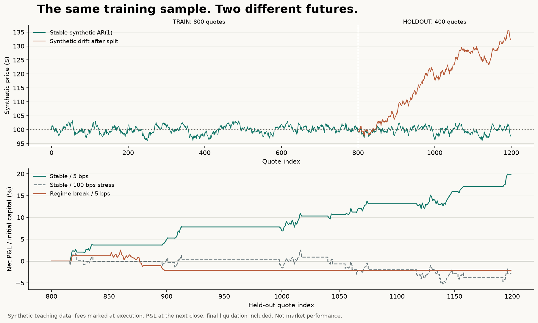
The chart shows why the formation sample cannot reveal the future regime. Its lower panel marks fees at the execution close and holding P&L at the following close, including final liquidation. It uses the implemented trading rules and costs, rather than plotting a theoretical forecast. All values are synthetic teaching outputs; the apparent stable-series gain is a feature of this constructed experiment, not a measured market opportunity.
Run the checked Python example
Save mean-reversion.py in an empty working directory and run python mean-reversion.py. The experiment uses Python’s standard library, with no pip dependencies or market-data service. It was executed and checked with CPython 3.14.0. For exact output reproduction, use the same Python version and the fixed seed 20261003; floating-point output is rounded in the table.
The script prints its parameter estimates and scenario table, then writes mean-reversion-results.json and mean-reversion-quotes.csv into your working directory. The published checked result file and generated quotes let you inspect the numbers independently.
Training estimates are frozen before the holdout. Every execution decision uses quote t−1, every interval P&L uses the position actually held from t to t+1, and final liquidation is charged. Assertions check that changing future observations cannot change earlier decisions, that the broken and stable samples produce identical training estimates, and that costs reconcile with turnover and the account balance.
#!/usr/bin/env python3
"""Original synthetic mean-reversion experiment for QuantSteps.

Run: python mean-reversion.py
Tested on CPython 3.14.0; standard library only, no pip dependencies.
Quotes 0..799 train parameters. Quotes 800..1199 are held out.
Signal at close t-1 fills at close t and earns only t..t+1 P&L.
One fixed unit; $100 initial research capital; arithmetic P&L / capital.
The final unit is liquidated at the last quote with its cost included.
This is a synthetic accounting exercise, not historical market evidence.
"""

import csv
import json
import math
import random
import statistics
from pathlib import Path

SEED = 20261003
N = 1200
SPLIT = 800
CAPITAL = 100.0
ENTRY_Z = 1.5
EXIT_Z = 0.25
STOP_Z = 3.0
MAX_HOLD = 20


def make_paths():
    rng = random.Random(SEED)
    shocks = [rng.gauss(0.0, 0.6) for _ in range(N - 1)]
    stable = [100.0]
    broken = [100.0]
    for t, shock in enumerate(shocks, 1):
        stable.append(100.0 + 0.9 * (stable[-1] - 100.0) + shock)
        if t < SPLIT:
            broken.append(stable[-1])
        else:
            broken.append(broken[-1] + 0.12 + shock)
    return stable, broken


def fit_training(prices):
    train = prices[:SPLIT]
    lag, current = train[:-1], train[1:]
    xbar, ybar = statistics.mean(lag), statistics.mean(current)
    phi = sum((x - xbar) * (y - ybar) for x, y in zip(lag, current))
    phi /= sum((x - xbar) ** 2 for x in lag)
    intercept = ybar - phi * xbar
    if not 0.0 < phi < 1.0:
        raise ValueError("Training fit does not support monotone AR(1) decay")
    return {
        "phi": phi,
        "mu": intercept / (1.0 - phi),
        "scale": statistics.stdev(train),
        "half_life": math.log(0.5) / math.log(phi),
    }


def run_backtest(prices, fitted, cost_bps):
    unit, age = 0, 0
    gross, costs, turnover = 0.0, 0.0, 0.0
    entries, exits, exposed = 0, 0, 0
    equity, peak, drawdown = CAPITAL, CAPITAL, 0.0
    rows = []
    for t in range(SPLIT, len(prices) - 1):
        # Only yesterday's quote enters today's execution decision.
        z = (prices[t - 1] - fitted["mu"]) / fitted["scale"]
        old = unit
        if unit:
            converged = (unit == 1 and z >= -EXIT_Z) or (unit == -1 and z <= EXIT_Z)
            adverse = (unit == 1 and z <= -STOP_Z) or (unit == -1 and z >= STOP_Z)
            if converged or adverse or age >= MAX_HOLD:
                unit, age = 0, 0
        elif ENTRY_Z <= abs(z) < STOP_Z:
            unit = -1 if z > 0.0 else 1
            age = 0
        # No same-close reversal/re-entry after an exit.
        if old == 0 and unit != 0:
            entries += 1
        if old != 0 and unit == 0:
            exits += 1
        traded_notional = abs(unit - old) * prices[t]
        fee = traded_notional * cost_bps / 10000.0
        pnl = unit * (prices[t + 1] - prices[t])
        gross += pnl
        costs += fee
        turnover += traded_notional / CAPITAL
        # Execution cost creates an equity mark before the next holding P&L.
        equity -= fee
        peak = max(peak, equity)
        drawdown = max(drawdown, peak - equity)
        equity += pnl
        peak = max(peak, equity)
        drawdown = max(drawdown, peak - equity)
        if unit:
            age += 1
            exposed += 1
        rows.append({
            "execution_index": t, "signal_index": t - 1,
            "price": prices[t], "z_from_previous_close": z,
            "units": unit, "gross_pnl": pnl, "cost": fee,
        })
    liquidation = abs(unit) * prices[-1]
    costs += liquidation * cost_bps / 10000.0
    turnover += liquidation / CAPITAL
    equity -= liquidation * cost_bps / 10000.0
    drawdown = max(drawdown, peak - equity)
    exits += int(unit != 0)
    assert entries == exits, "Every entry must have a completed exit"
    assert math.isclose(costs / CAPITAL, turnover * cost_bps / 10000.0, abs_tol=1e-12)
    assert math.isclose(equity, CAPITAL + gross - costs, abs_tol=1e-10)
    return {
        "cost_bps": cost_bps, "gross_pct": gross / CAPITAL * 100.0,
        "cost_pct": costs / CAPITAL * 100.0,
        "net_pct": (gross - costs) / CAPITAL * 100.0,
        "turnover_x": turnover, "round_trips": entries,
        "exposed_pct": exposed / len(rows) * 100.0,
        "max_drawdown_pct_initial": drawdown / CAPITAL * 100.0,
    }, rows


def checks(stable, broken, fitted):
    assert stable[:SPLIT] == broken[:SPLIT]
    assert fit_training(broken) == fitted
    result, rows = run_backtest(stable, fitted, 5.0)
    changed = stable.copy()
    changed[1000:] = [p + 100.0 for p in changed[1000:]]
    _, changed_rows = run_backtest(changed, fitted, 5.0)
    # A future perturbation cannot alter earlier decisions or earlier P&L.
    assert rows[:199] == changed_rows[:199]
    assert [r["units"] for r in rows[:201]] == [r["units"] for r in changed_rows[:201]]
    assert all(r["signal_index"] < r["execution_index"] for r in rows)
    # Hand-check the first interval's fixed-unit accounting.
    first = rows[0]
    expected = first["units"] * (stable[SPLIT + 1] - stable[SPLIT])
    assert math.isclose(first["gross_pnl"], expected, abs_tol=1e-12)
    assert math.isclose(result["net_pct"], result["gross_pct"] - result["cost_pct"], abs_tol=1e-12)
    # A profitable next interval must not conceal the entry-fee equity dip.
    fee_dip_prices = [100.0] * 799 + [150.0, 150.0, 100.0, 100.0]
    fee_dip, _ = run_backtest(fee_dip_prices, {"mu": 100.0, "scale": 30.0}, 100.0)
    assert math.isclose(fee_dip["gross_pct"], 50.0, abs_tol=1e-12)
    assert math.isclose(fee_dip["cost_pct"], 2.5, abs_tol=1e-12)
    assert math.isclose(fee_dip["max_drawdown_pct_initial"], 1.5, abs_tol=1e-12)


def main():
    stable, broken = make_paths()
    fitted = fit_training(stable)
    checks(stable, broken, fitted)
    scenarios = []
    for name, path, cost in [
        ("Stable AR(1)", stable, 5.0),
        ("Stable AR(1), cost stress", stable, 50.0),
        ("Stable AR(1), extreme cost stress", stable, 100.0),
        ("Random walk with drift after split", broken, 5.0),
    ]:
        stats, rows = run_backtest(path, fitted, cost)
        scenarios.append({"scenario": name, **stats})
    print("Synthetic example; arithmetic P&L / $100 initial capital")
    print("Training fit:", json.dumps(fitted, sort_keys=True))
    print("scenario | cost bps | gross % | cost % | net % | turnover x | round trips | DD % initial")
    for s in scenarios:
        print(f"{s['scenario']} | {s['cost_bps']:.0f} | {s['gross_pct']:.4f} | "
              f"{s['cost_pct']:.4f} | {s['net_pct']:.4f} | {s['turnover_x']:.4f} | "
              f"{s['round_trips']} | {s['max_drawdown_pct_initial']:.4f}")
    print("Checks passed: training isolation, future perturbation, execution lag, costs, fee-dip drawdown, liquidation.")
    output = Path.cwd()
    (output / "mean-reversion-results.json").write_text(
        json.dumps({"synthetic": True, "seed": SEED, "training": fitted, "scenarios": scenarios}, indent=2),
        encoding="utf-8",
    )
    with (output / "mean-reversion-quotes.csv").open("w", newline="", encoding="utf-8") as f:
        writer = csv.writer(f)
        writer.writerow(["index", "stable_price", "regime_break_price", "sample"])
        for i, (a, b) in enumerate(zip(stable, broken)):
            writer.writerow([i, a, b, "train" if i < SPLIT else "holdout"])


if __name__ == "__main__":
    main()
Notice that an entire list of synthetic quotes exists in memory. That alone is not leakage; leakage occurs when future values enter a parameter, candidate selection, decision or supposed earlier outcome. The indexing and the perturbation assertions make that distinction inspectable. The assertions support these stated mechanics, but cannot establish that a real-market dataset or fill model is appropriate.
Checked gross returns, costs and net results
These percentages are arithmetic P&L divided by $100 initial research capital. The example holds fixed units, so it does not compound position weights or report a CAGR. Total turnover is the sum of absolute executed dollar notional divided by that same initial capital. A complete entry and exit around a $100 price contributes about 2× turnover.
Scroll horizontally to read every column.
| Synthetic holdout | Cost per executed dollar | Gross P&L / initial | Cost / initial | Net P&L / initial | Total turnover | Completed round trips |
|---|---|---|---|---|---|---|
| Stable AR(1) | 5 bps | 21.0744% | 1.1942% | 19.8802% | 23.8834× | 12 |
| Same stable quotes | 50 bps stress | 21.0744% | 11.9417% | 9.1327% | 23.8834× | 12 |
| Same stable quotes | 100 bps extreme stress | 21.0744% | 23.8834% | −2.8090% | 23.8834× | 12 |
| Random walk with drift after split | 5 bps | −1.7138% | 0.4100% | −2.1237% | 8.1996× | 4 |
At 5 bps, 23.8834 × 0.0005 = 0.0119417 of initial capital, or 1.19417%. Subtracting that cost from 21.0744% gross gives 19.8802% net. The break-even proportional cost for this fixed trade list is approximately 88.24 bps per executed dollar. That calculation assumes changing costs does not change fills or decisions.
The 50 and 100 bps rows deliberately stress the cost assumption. They are not estimates for a broker or asset. The extreme row makes the distinction between a correct directional hypothesis and a profitable implementation explicit. With the same quotes, decisions and gross P&L, costs alone change the conclusion.
The regime-break row fails for a different reason. The earlier equilibrium and persistence estimates remain identical, but later prices no longer follow the assumed correction mechanism. The entry band and stop rule eventually keep the system out of very large deviations, limiting further exposure without making its earlier losing trades profitable.
Maximum peak-to-trough loss measured against initial capital is 2.5016% for stable/5 bps, 3.3766% for stable/50 bps, 7.8139% for stable/100 bps, and 4.6236% for the drifted/5 bps case. The account is marked immediately after execution costs, then again after the following holding interval, and after terminal liquidation. This keeps a subsequent gain from concealing the entry-fee equity dip. Intrabar loss could be larger. Avoid reading a low synthetic drawdown as a real risk estimate.
Audit the timeline and the accounting
Suppose close 899 produces an eligible long signal. The implementation executes at close 900 and first earns price(901) − price(900). It does not earn the move from 899 to 900. The exit follows the same rule: a convergence observation at close 905 changes the holding at close 906, after the strategy has remained exposed during 905→906.
Scroll horizontally to read every column.
| Time | Information or action | Exposure used for P&L |
|---|---|---|
| Close t−1 | Observe quote and compute signal | The new decision earns no preceding price move |
| Close t | Execute the previously computable decision and charge turnover cost | Updated unit begins the next holding interval |
| Close t+1 | Mark the position’s price change | unit(t) × [price(t+1) − price(t)] |
| Final close | Liquidate remaining units and charge cost | No new speculative trade is opened |
A different next-open or delayed auction implementation needs different quotes and return intervals. Applying a generic “shift(1)” without identifying its fill convention can still create an impossible execution. The key is to state when data becomes available, when an order could be submitted, and which prices are actually tradeable.
For pairs, use holdings and instrument prices directly. If the unit spread uses positive beta, a long spread holds qY = +1 and qX = −beta. Over the holding interval, gross P&L is qY × change(Y) + qX × change(X). Trading cost depends on |change(qY)| × Y + |change(qX)| × X, with each leg’s own cost rate where appropriate. Include both entry and exit, hedge rebalances, borrow and financing, and delays or partial fills.
Alpha is a fitted intercept in the reference; it is not a security whose quoted price can be bought. A log-price spread also does not directly define share holdings: an implementation needs a dollar-exposure rule and its own P&L accounting. Avoid dividing a zero-crossing spread by its previous level to invent a percentage return.
If coefficients update, changes in the fitted residual can come from the model moving rather than the held assets earning P&L. Reconcile the trade ledger independently of the residual chart. The free trading-cost sensitivity tool illustrates turnover deductions; it does not execute trades or estimate market-specific fees.
What makes a convincing-looking backtest fail?
A full-history hedge ratio can let later relationships improve earlier signals. A full-history mean or scale can do the same. Selecting today’s surviving stocks excludes failures, and choosing a pair because you already saw its later convergence leaks through selection even if the subsequent calculation uses lagged data.
Use formation dates, point-in-time instruments and timestamped inputs. Keep a record of rejected candidates and failed parameter sets. If you revise a threshold after seeing holdout results, that period becomes development evidence; use a new evaluation period for the revised rule. A chronological split is necessary, but does not by itself remove every leak.
Trading failure can also survive perfect code. An apparent negative short-lag return correlation can reflect bid–ask bounce rather than accessible midpoint movement. Sparse instruments may print stale prices. Short availability may disappear exactly when the signal is largest. Costs and impact may rise during the dislocation. Simultaneous exits by other traders can widen the spread rather than close it.
Declare exposure limits, time limits, acceptable drawdown and pause conditions before evaluating the strategy. A failed stability diagnostic can trigger no new entries; it cannot guarantee a favorable exit from existing positions. Avoid automatically increasing size when the gap widens. A larger deviation may contain new information about the failure of the reference.
Review the worst trades and longest holding periods, not only the win rate. A strategy can win often yet lose money if its occasional loss is large. Report exposure, turnover, gross and net results, cost sensitivity, parameter stability and results across separate later periods. For dependent observations, uncertainty estimates must respect the time-series dependence rather than pretending every bar is an independent trade.
A practical workflow for your own mean reversion study
- State a falsifiable claim. Name the variable, reference, horizon and reason correction might occur. Write what would count against it before viewing the evaluation period.
- Audit the data. Check units, calendars, missing quotes, corporate actions, lookback availability and the instrument universe as it existed at each date. Align both legs of a pair.
- Reserve later observations. Use an earlier formation sample to select candidates and estimate parameters. Put threshold exploration in a declared development process. Keep the final evaluation period separate.
- Examine the process. Plot levels, changes and residuals. Use appropriate stationarity and cointegration diagnostics with declared specifications. Evaluate half-life and parameter stability without treating them as profitability tests.
- Write an execution specification. Define signal availability, order submission, price convention, delay, size, entry, exit, stop, time limit and terminal liquidation. For pairs, write both share or dollar holdings.
- Reconcile a few trades by hand. Recalculate the earliest entry and exit, both legs’ P&L, and their traded notional. Confirm that increasing future quotes cannot change an earlier decision.
- Evaluate net outcomes. Include a realistic range of spread, fees, impact, borrow and financing assumptions. Compare a no-trade and an appropriate exposure baseline. Separate cost failure from hypothesis failure.
- Document uncertainty. Save the dataset version, code, declared parameters, candidate history, failed cases and interpretation. Decide whether the evidence supports further research, a revision or rejection.
The positions and turnover lesson is a Pro lesson for practising how holdings produce costs. You can complete every calculation in this public article with the downloadable script; the lesson is an optional continuation.
Knowledge checks with worked answers
1. Is the intercept the equilibrium?
An AR(1) is X(t+1) = 6 + 0.80 × X(t) + epsilon. What is its stable mean, and the next expected value from 40?
Answer: mu = 6 / 0.20 = 30. The next conditional expectation is 6 + 0.80 × 40 = 38. The gap falls from 10 to 8. Its half-life is log(0.5) / log(0.80), approximately 3.11 observations.
2. Did a closing gap make the short profitable?
A price jumps from 100 to 120 and remains at 120. A moving average rises from 100 to 120. The plotted price-minus-average gap closes. Does that prove a profitable short?
Answer: No. A short filled at 120 and covered at 120 has zero gross price P&L and negative net P&L after costs. The average moved; the held security did not provide the expected reversal.
3. Which return belongs to the signal?
A signal formed at close 20 is executed at close 21. The price is 100 at close 20, 98 at close 21 and 99 at close 22. What is the first one-unit long P&L before cost?
Answer: $1, earned from the actual fill at 98 to the next mark at 99. The −$2 move before the fill does not belong to the new position. Entry cost is based on $98 of executed notional, and closing the unit later incurs another cost.
4. Can a profitable gross result be untradeable?
A fixed-unit strategy earns 4% gross on initial capital and generates 40× total turnover. Combined proportional cost is 12 bps per executed dollar. What is net P&L?
Answer: Cost is 40 × 0.0012 = 0.048, or 4.8% of initial capital. Net P&L is −0.8%, before any separately omitted financing. This is why reporting gross returns or a high win rate does not finish the research question.
5. Does changing tomorrow’s price change today’s fitted equilibrium?
In the shipped example, replace all holdout prices after index 1,000. Should the fit or any execution decision through index 1,000 change?
Answer: The training fit must remain unchanged. Execution at 1,000 uses quote 999, so that decision must also remain unchanged. Its subsequent P&L can change because quote 1,001 changes. Distinguish an immutable past decision from an outcome that legitimately depends on a future price.
Frequently asked questions
Is “mean reverted” a valid expression?
Yes, as a past-tense description such as “the spread mean reverted toward its fitted average.” Mean reversion is the name of the concept, and mean-reverting describes an assumed process property. An observed correction does not establish that the process reliably repeats it.
Do all stocks eventually return to their historical average?
No. Growth, corporate change, default and new information can make an old price level irrelevant. A price can remain nonstationary while returns or a carefully defined residual have different properties. State which variable and horizon you mean before testing the claim.
Is mean reversion the same as regression to the mean?
They are related but distinct uses of “return toward average.” Regression to the mean can arise when extreme observations contain temporary noise, so a subsequent measurement is less extreme without a physical correcting force. A mean-reverting time-series model specifies conditional dynamics. Neither phrase alone proves a trading edge.
What is the formula for the mean-reverting level?
For X(t+1) = c + phi × X(t) + epsilon with a stable AR(1) and zero-mean innovations, the long-run mean is c / (1 − phi). The conditional forecast h observations ahead is mu + phi^h × [X(t) − mu]. A moving-average reference is a different estimation choice.
Does an ADF p-value below 0.05 prove profitability?
No. It is evidence against a unit root under the stated regression, lag and sample specification. Profitability also depends on selection, parameter stability, signal timing, fills, sizing and costs. Multiple candidate tests require attention to false discoveries.
Is a Hurst exponent below 0.5 enough to identify a mean-reverting market?
No. Antipersistence under a scaling model is not a universal certificate of a stable mean or tradeability. Specify the estimator, levels versus increments, scales and sample. Short-memory dependence and finite samples can distort a simple Hurst interpretation.
Which time frame is best for mean reversion?
There is no universally best time frame. The relevant horizon must suit the variable’s estimated dynamics, fill delay, costs and funding constraints. A short half-life can disappear before execution, and a long half-life can require an impractical holding period. Compare declared horizons on later data.
Is the downloadable example a historical backtest?
No. It is an original synthetic experiment with a fixed seed and an intentionally changed holdout regime. It demonstrates training-only estimates, delayed fills, turnover, costs and failure. It contains no market-performance claim and needs no paid course or data subscription to run.
Sources and methodology
Sources checked Oct 3, 2026. Original exercises and synthetic examples are identified in the text. Employer disclosures, catalog records and technical documentation retain their own dates and limitations.
- Forecasting: Principles and Practice — autoregressive models
Author-maintained textbook explanation of AR models and the conditions for stationarity. Numeric examples and research code in this article are original.
- Forecasting: Principles and Practice — stationarity and differencing
Distinguishes nonstationary levels from stationary changes and describes random-walk behaviour.
- MIT OpenCourseWare — the Ornstein–Uhlenbeck semigroup
University lecture reference for the continuous-time OU setting. The half-life and forecasts shown here follow from the stated conditional-mean formula.
- statsmodels — adfuller
Official ADF API documentation: unit-root null, deterministic regression choices, lag selection and returned statistics.
- statsmodels — coint
Official augmented Engle–Granger documentation: no-cointegration null, integration-order assumption and residual-based inference.
- Andrew W. Lo — Long-Term Memory in Stock Market Prices
Original NBER Working Paper 2984 (1989), subsequently published in Econometrica (1991). Modified R/S analysis accounts for short-range dependence.
- John Bollinger — Bollinger Band rules
The indicator creator’s guidance explains why a band tag by itself is not a reversal instruction and why prices can follow bands in trends.
- Investor.gov — Updated Investor Bulletin: Exchange-Traded Funds
SEC investor education on authorized participants, creation/redemption and premiums or discounts. Cited for ETF mechanics, not a claim of attainable profits.